


Our models are based upon the fukui & Ishibashi (FI) traffic flow mrodel in which cars are allowed to move amaximum of (M) sited in each time step if spacing permits, together with aprobilstic delay for the cars moving out the maximum speed.
We propose & study now vehicular traffic flow models, incorporating the anticipation of the change in the car spacings ahead in the determinetion account the anticipation in each timestep. By taking in to account the change of car spacing due to moment of the car ahead, the present models give an enhanced traffic flux as compared to the fukui & Ishibashi model. The present model also afundamental diagram consisting of there phases — afeature consistent with traffic flow observations.
Key words: trffic flow, ceunlan automation automation models.
Vehicular traffic flow problems have attracted much attention in the physics community in recent years.(1–4) Fundamentally, these problems are related to a general class of problems in physics called driven diffusive systems.(4–5) Practically, recent developments in cellular automaton (CA) models of traffic, flow provide a novel approach to the complicated problems of vehicular traffic flows. Nagel and Schreckenberg (NS)6 proposed a CA model for traffic flow in one dimension in which cars are allowed, to accelerate gradually up to a maximum speed with a built-in probabilistic delay to model the complexity in the drivers' behavior. The model gives a fundamental diagram, i.e., flux as a function of car density, similar to that observed in traffic flow data3–7 As a CA model, the NS model can be readily studied via numerical simulations. CA models for one lane form the basic components in building a CA model for traffic flow in cities. Nowadays, large projects have been set up to simulate traffic flow in cities,2–8 for example, in Dallas and in Seattle. This new approach complements the conventional approaches based on kinetic theory and the fluid dynamical approach.3–4-9 The NS model, while attracting much attention due to its simplicity and nontrivial features, does not present all the features observed in real traffic flow. For example, there are observations indicating a hysteresis effect in which the speed may take on different values with respect to car concentration depending on whether the car density is increasing from a dilute phase or decreasing from a concentrated phase.10–11 In addition, there are empirical results showing that there are three phases in the fundamental diagram3 namely, the free-flow phase for low car densities, the stop-and-go phase at high densities, and the synchronized phase at intermediate densities. The NS model does not reproduce these features clearly. Moreover, even with the optimized value of the speed limit of 5 sites per time step corresponding to the best fit to empirical results,3 the flux in the NS model is found to be lower than that in real traffic flow.
Fukui and Lshibashi (FI)2 proposed a slightly simpler CA traffic flow model in which the cars are allowed to accelerate rapidly instead of gradually as in the NS model. In addition, probabilistic delay only applies to the cars moving at the highest allowed speed so as to model the fact that drivers tend to apply the brake more often when they are travelling near the speed limit. The model.gives a fundamental diagram similar to that of the NS model. As both of the changes in the FI model tend to increase 'the speed, the maximum flux is therefore higher. With the simplified CA rules, the FI models can be treated analytically by mean hield theories. Wang and co-workers have developed mean field theories based on the time evolution on the occupancy of the sites on the road3 and on the car spacings. These theories give results in good agreement with those obtained by numerical simulations. The NS model has also been studied by mean field theories.15–16
Recently. Li et al.17 proposed and studied numerically a modified NS model in which the anticipated movement of the car in front is incorporated. Interestingly, the maximum traffic flux was found to be higher than that of the basic NS model, thus the modified model better represents the empirical results obtained from observations. The modified model also gives the hysteresis effect in the fundamental diagram when no probabilistic delay effect is imposed. It is, therefore, interesting to study how the consideration of the anticipated movement of the car ahead affects the features in the FI model. In this work, we study numerically the dependence of the traffic flux as a function of car density for modified FI models in which the anticipated change in the car spacing is incorporated. Results are compared with those obtained in the basic FI model. With a conservative anticipation scheme, the fundamental diagram is found to have three distinguishable phases. The low-density phase gives a linear dependence of the flux on the density.
The high-density phase gives a decrease of the flux on the density similar to the basic FI model, as the effect of changing car spacing 'diminishes when the car density is high. At intermediate densities, the flux drops more rapidly with density when compared with the high-density phase. The maximum flux is higher than that in the FI model. A more aggressive anticipation scheme gives an enhanced flux for a wide range of car densities.
Our models basically follow that of Fukui and Ishibashi. Consider a one-dimensional road with a single lane consisting of L sites. Let.V be the number of cats on the road. The cars are assumed to be travelling to the right. The cars'are labelled (n=1,2,-N)v> from right to left. Hence the number density of cars is given by p = N/L. In a CA model, the motions of the cars follow a set. of parallel updating rules. A car is allowed to move a maximum of M sites in a time step if the spacing in front of the car permits. Thus M. serves as the speed limit in' the model. In the FI model, the spacing;s simply determined by the spacing at the current time step, without consideration of the fact that the car in front would also move in the next time step. In the present models. drivers anticipate the motion of the car ahead and decide the speed according to the spacing at the current time step and the anticipated motion. At each time step, the anticipated motion of the car ahead is predicted using the basic FI model. To avoid collisions, the anticipated motion is only allowed to take on at most (M — 1) sites. The actual motion of the car ahead, of course, could be different from the anticipated motion. This predicted motion has the effect of enhancing the car spacing in front so that the driver can take advantage of it and travel at a higher speed. For a car with a spacing that allows it to actually travel at the maximum speed M, there is a probability f that it will travel at a speed M — 1. The parameter/ thus gives a probabilistic delay for fast moving cars, as in the FI model. It models the feature that drivers travelling at maximum speed are more cautious, for safety reasons or simply to avoid speeding.
Let.xn(t) and vn(t) be the position and speed of the n-bh car at time respectively. The spacing at time t is. therefore, given by
dn(t) = xn-1(+)-xn(4)-1 (1)
Model A: A more conservative anticipation scheme is given by the following steps.
Step 1: Anticipation of motion — The anticipated motion of the in — l)-th car in front of the n-th car is represented by an anticipated speed vn-1(t+1), which is determined by the basic FI model. To avoid collisions and to allow for wider spacing between cars, an anticipated motion up to only (m-1) sites is allowed. Thus.
Vn-1 (t+1) =min (m-18 max (odn-1(t)-1) (2)
Step 2: Deteiwiination of actual speed — The actual speed of the n-th car is determined by the current spacing and the anticipated motion of the car in front. Probabilistic delay is applied only to cars that are allowed to move at the speed limit. Therefore, with probability (1 —f),
Vn(t+1)=min)m,dn (t) +vn-1(t-1) (3)
With probability f, vn(t+1) =min (m-1, dn(t)+vn-r(t+1). (4)
Step 3: Position Update — The position of each car is then updated according to
x(t + 1) = Xn(t) + Vn (5)
Equations (3), (4), and (5) give'a set of equations for the time evolution of Model A.
Model B: To avoid collisions, it would be sufficient to replace the anticipated speed in eq. (2) by
Vn-1(t+1) = min {m-1,max{0,dn -1(t)}} (6)
Equation (6) would in general lead to a higher speed in Model B than'in Model A. Equations (3), (4). (5) with vn- (t+1)) as defined in eq. (6) constitute the set of equations for the time evolution of Mode! B.
In both the NS and FI models, each site models the minimum length that a car occupies on the road.It has been shown that taking M = 5 gives the best description of real traffic flow as it reasonably models the speed limit. In traffic flow problems, the most interesting relation to study is the fundamental diagram, which gives the traffic flux as a function of car density. The traffic flux is the average number of cars passing through a location in a unit time and is'simply given by the product of the average speed and the car density. Figure 1 shows the fundamental diagram obtained by numerical simulations for Model A with M = 1.2,..., 5 and a random delay probability of f = 0.3. We used a lane of 1000 sites, with periodic boundary conditions imposed. The results are obtained in the long time limit when the flow approaches its steady state. For comparison, we include the results for the basic FI model with the same sets of parameters in Fig. 1. The distinguishable features, as compared to the FI model, are that the present model allows a higher maximum traffic flux and there exist three ranges of car densities corresponding to different flux behavior.
For concreteness, we focus our discussion on the case of M = 5. The maximum flux in this case is about 1.15, corresponding to a car number density of about 0.275. This implies that the average speed is about 4.18 sites per time step. The flux is significantly higher than the maxiumum flux of about 0.80 corresponding to a car number density of 0.20 for the basic FI model. The increase in the flux is due to the fact that with drivers anticipating the movement of the car ahead, the cars can attain a higher average speed in the present model. Figure 1 also shows that the effects of including the anticipation of car motion are only significant in an intermediate range of car densities. For low car densities, cars are well separated in the long time limit. If the density is sufficiently low so that the spacing between cars is larger than M, then anticipation becomes unneccessary as the cars can always travel at the speed limit. Hence the flux in Model A becomes identical to the FI model for a range of densities below 0.15 for M = 5. For high car densities, p > 0.5, some of the cars are blocked by the car in front. When a car is following another car that is blocked in front. the anticipation of motion does not change the speed of the car from that of the basic FI model since the car in front is anticipated to remain stationary. Hence for M ≥ 2, the flux in Model A is the same as that of the FI model for p > 0.5. i; should also be noted that for p > 0.5. the flux becomes independent of M for M ≥ 2. This is because for p > 0.5, the density is so high that the cars are either blocked in front or there is only one empty site in front. Therefore, the cars simply cannot move [see eq. (2)] at the allowed speed limit m these congested cases, and the results become insensitive to M. For the special case of M = 1, cars are only allowed to move one site at most in each time step. Therefore, anticipation cannot make the car move faster, and hence Model A and the FI model give identical results. It is found that Model B also gives similar features. The enhanced maximum flux is somewhat higher than the observed value.3 figure 2 shows the corresponding average speed of cars as a function of car number density for Model A for different values of M. As in the fundamental diagrams, the speed shows three different regimes of dependence on the number density, with the regimes in low and high densities exhibiting features similar to the basic FI model.
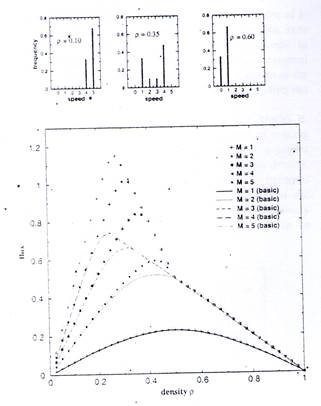
Fig. I. Fundamental diagram (lower panel) of Model A (symbols) showing the traffic flux as a function of car number density for different values of \t. The probability of random delay is taken to be / = 0.3. Results for the basic FI model (lines) are included for comparison. Model A shows a synchronized phase at a range of intermediate densities. The upper panel shows the distribution of speeds among the cars in M = 5 for three different densities corresponding to the free-flow phase (p = 0.10). the synchronized phase (p = 0.35), and the stop-and-go phase (p = 0.60). respectively.
The most interesting feature in the fundamental diagram (Fig. 1) is that there are three different ranges of car densities with different behavior. For small p, there is a range in which the flux increases almost linearly with car den: ity. In this range, the cars can attain a high speed and the flux is basically determined by the density. With anticipation, high speed is attained to a higher car density than in the FI model for A ≥ 2. In the upper panel of Fig. 1, we show the distribution of speeds among the cars for the case of M = 5. The distribution is normalized so that all the frequencies of occurrence of the speeds add up to unity. Thus, the bars in the figure give the probability of a'car having a certain speed. The distribution at low density {e.g., p = 0.10) shows that most of the cars move at the highest possible speed (M = 5) with a small fraction at the speed (m— 1) due to probabilistic delay. The ratio of the' occurrence of speeds M and' (M — 1) is 7/3. as expected for f = 0.3. Thus, the spacings between cars are always larger than M in this phase. This corresponds to the free-flow phases) in which there is no blockage of cars. The free-flow phase extends to a higher car density in Model A (up to p ~ 0.30) as cars can still move with speed.m/ at densities for which the basic FI model already exhibits a blockage of cars. In an intermediate range of densities, blockage between cars becomes more pronounced because of the higher speed of the cars • and the fact that anticipations depend on spacings. Both of these factors lead to a more sensitive dependence of the speed on car densities in this intermediate range.as shown in Fig. 2.
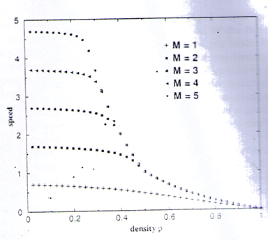
Fig. 2: Average speed as afunction of deusty of car for model A for differed value of m-the probability of random delay is taken to be f = 03
The drop in flux with car density beyond the maximum flux is due to a steep drop in average speed. It should be noted that over this intermediate range of car densities, the flux is higher than the basic FI model. The appearance of the feature in the intermediate range can be recognized as the synchronized phase observed in real traffic flow. In the synchronized state, the drivers have self-organized themselves into a phase in which the cars are, in general, moving, but at a lower speed.3' The upper panel of Fig.1 shows the corresponding distribution of speeds for a density (p = 0.35) in the synchronized phase. The distinguished features are that there is a spread in the speeds ranging from 1 to (M — 1) and all the cars are constantly in motion. It should be noted that the basic FI model only shows a naiTow intermediate range of densities with this feature. For high car densities, anticipation becomes ineffective and the results obtained are identical to those of the FI model. Figure 1 (upper panel) also shows that, in the high-density regime (p > 0.5), some of the cars are blocked during the flow and some take on the low speed of 1.
This leads to the nonvanishing probability of having zero speed. Therefore, the high-density phase corresponds to stop-and-go traffic3 which is characterized by the occasional blockage of cars in the Bow. The fundamental diagram of the present modej is. Therefore, compatible with that observed empirically in real traffic flow.
Figure 3 shows the fundamental diagram of Model B, which corresponds to a more aggressive scheme of making use of the anticipated motion. Model B gives a- higher maximum flux than Model A at a slightly higher car density. From. eq. (6), it is expected that the flux becomes independent of M (M ≥ 2) only for p ≥ 2/3 when the blockage of cars becomes effective. In the high-density limit, the flux is given by 2(1 — p), which is twice that in the basic FI model.14 The upper panel in Fi.g. 3 shows the corresponding distributions of speeds typical of the three different phases.
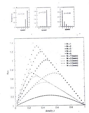
Fig. 3. Fundamental diagram (lower panel) of Model B (symbols) for ferent values of M The probability of random delay is taken to be = 0.3. Results for the basic FI model (lines) are included for mparison. The high-density regime sets in for p > 2/3. The upper ncl shows the distribution of speeds among the cars in V/ = 5 for three '•-•rent densities corresponding to the free-flow phase (p = 0.10). the nchronizcd phase (p — 0.35). and the stop-and-go phase (p = 0.80).
The distributions of Model A and Model B are identical in the low-density regime. In the intermediate density range. Model B has a higher fraction of cars moving at the speed (M — 1), while Model A has a wider spread of speeds as a result of its more conservative anticipation scheme. In the high-density regime. Mode! B has a small fraction of cars moving at higher speeds (v >1) as.a result of anticipation, leading to the enhanced flux.. In summary..we presented numerical results of the. effects of anticipation of the movement of the car ahead on the FI model. The models are more realistic in that cars can move collectively at high speed on highways. The spacing between cars is usually governed by the stopping distance rather than the' speed limit. It is shown that with anticipation incorporated, the fundamental diagram clearly exhibits a free-flow phase at low car densities, a.synchronized phase a; intermediate densities, and a stop-and-go phase at hign densities. The results are consistent with features observed in real traffic flow.
References:
1. Traffic ami Granular Flow '97, ed. M. Schreckenberg and D. E. Wolf (Springer, Singapore, 1998).
2. D. Helbing, H. j. Herrmann. M. Schreckenberg and D. If. Wolf: Traffic and Granular Flow '99: Social, Traffic and Granular Dynamic (Springer, Berlin, 2000).
3. D. Chowdhury. L. Santcn and A. Schadschneidcr: Phys. Rep. 329 (2000) 199
4. D Helbing: Rev. Mod. Phys. 73 (2001) 1067.
5. B. Schmittmann and R. K. P. Zia: Phase Transitions and Critical Phenomena, ed. C. Domb and). L. Lcibowilz (Academic Press. San Diego, 1995) Vol. 17.
6. K. Nagel and M. Schreckenberg:) Phys. 1 (france) 2 i 1992) 2221
7. F. L. Hall, B. L. Allen and M. A. Gunter: Transport. Res, A 20 (1986) 197.
8. P. M. Simon and K. Nagel: Phys. Rev. E 58 (1998) 128b.
9. Prigogine and R. Herman: Kinetic Theory of Vehicular Traffic (EJscrvier, Amsterdam, 1971).
10. K. Nagel and M. Paczuski: Phys. Rev, If 51 11995) 2090.
11. S. Krauss, P. Wagner and C. Gawron: Phys. Rev. E 55 (1997) 5597,
12. M. Fukui and Y. Ishibashi: J. Phys. Soc.)pn. 65 (1996) 1868.
13. B. H. Wang, Y. R. Kwong and P. M. Hui: Phys. Rev. E 57 (1998) 2568.
14. B. H. Wang, L. Wang, P. M. Hui and B. Hu: Phys. Rev. E 58 (1998) 2876.
15. A. Schadschneider and M. Schreckenberg: J, Phys, A 30 (1997) L69
16. A. Schadschneider: Eur. Phys. J, B 10 (1999) 573.
17. X. Li. Q. W'u and R. Jiang: Phys. Rev. E 64 (2001) 066128.
