Introduction

The growing demand for energy production and the optimization of related processes have led to the construction of increasingly complex wellbores. In particular, extended reach horizontal wellbores are required to access distant resources from existing facilities. This results in longer sections where drilled cuttings can settle, thereby challenging cuttings removal efficiency. In horizontal wells, the primary driving force governing transport phenomena is dragging, whereas lifting plays a more limited role (Bizhani and Kuru, 2018). To effectively remove deposited cuttings through either dragging or lifting, achieving—and ideally exceeding—the critical flow velocity and shear stress threshold for bed erosion becomes essential (Li and Luft, 2014). The calculation of critical flow velocity typically relies on fluid property models (Okesanya et al., 2020).

For the internal cuttings bed property measurements with the granular rheometer cell, the samples must be pre-consolidated. This is normally called “pre-shear” and is performed applying a rheometer operator defined maximum normal stress, depending on the particle size, shape and operational conditions. Then at a constant rotational speed, “shear-to-failure” points of reduced normal stress between 30 and 80 % of the maximum load are performed, which will result in the bed breaking and starting to flow again. The pre-shear is done to get the sample into a repeatable state, but also at this process already is yielded information on the bed behavior under the pre-compaction stress.

The two measurements stages per cycle, “pre-shear” and “shear-to-failure” are repeated two or more times at varying conditions to record necessary data for the analysis, obtaining the yield locus as an extrapolated line from the failure points. Two measuring cycles are shown in Fig. 1a) is shown the “pre-shear” at a pre-set maximum normal stress and the “shear-to-failure” stresses observed at 30 % and 80 % of this pre-set maximum normal stress. These “shear-to-failure” stresses are plotted to obtain the yield locus as it is shown in Fig. 1b). The yield locus then, is used to obtain the Mohr-Coulomb failure envelop providing the information of the unconfined yield strength and the maximum principal stress.

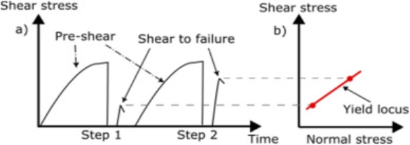
Fig. 1. Yield locus definition from shear to failure measurement

Once the yield locus is determined, the two semi-circles are calculated through distinct methods. The first semi-circle is defined as having a tangent to the yield locus and crossing the origin axes. The second intersection point along the normal stress axis corresponds to the unconfined yield strength, which represents the maximum principal stress that causes the bulk material in an unconfined state to fail under shear. The second semi-circle also has a tangent to the yield locus but intersects at the pre-shear measured stress. Here, the initial intersection point with the normal stress axis signifies the major principal stress. These two semi-circles are illustrated in Fig. 2.

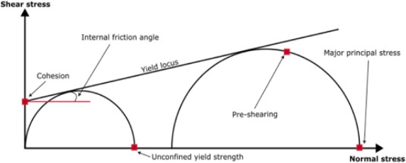
Fig. 2. Shematic diagram of powder yield locus

The measured results are analyzed using the Mohr-Coulomb criterion, in a similar manner as often used for rock mechanics characterization as describe by for example Fjær et al. (2008) which is shown in Eq. (1). To predict the required stress for the cuttings-bed to be disturbed. Hence, to optimally remove the drilled cuttings out of the wellbore.

2. Materials and methods

2.1. Materials

In the experiments, sand grains (quartz) of irregular shape, but from the same source with average size of 1.3 mm, sand grains were used to simulate the drilled cuttings as are the simplest type of rock formation down-hole. These particles were saturated in the first test with water. In the second test the particles were saturated with a common field applied inhibitive water-based drilling fluid with specific gravity of 1.5. This fluid contains KCl, soda ash, polyanionic cellulose, starch, xanthan gum, barite. Finally, in the last test a field applied oil-based drilling fluid with specific gravity of 1.5 containing base oil, CaCl ₂ , Clay, lime, fluid loss agents, emulsifiers, and barite was used.

2.2. Drilling fluid flow profile

The drilling fluids’ viscosity profile was characterized through a flow curve. The plotted data were derived from analysis performed with a rheometer Anton-Paar MCR102, equipped with a Couette geometry holding the temperature at 25 °C. The samples were initially pre-sheared at 1000 s-1 for 120 s to reach steady-state shear viscosity. After this, a measurement protocol was started ramping down from 1200 s to 1 to 60 s-1 in 100 logarithmic steps, followed by 5 logarithmic steps from 60 s to 1 to 10 s-1, and finally with 100 logarithmic steps from 10 s to 1 to 0.1 s-1. The measuring time per point was set to 2 s. As seen in Fig. 3. The specific gravity and the flow profile of both drilling fluids are quite similar, reaching a maximum difference at a shear rate of 94 1/s of 27 %.

References:

1. Abbas et al., 2021,A. K. Abbas, M. T. Alsaba, M. F. Al Dushaishi, Improving hole cleaning in horizontal wells by using nanocomposite water-based mud, J. Petrol. Sci. Eng., 203 (2021), Article 108619
2. Azar and Sanchez, 1997J. Azar, A. Sanchez, Important Issues in Cuttings Transport for Drilling Directional Wells, SPERio de Janeiro, Brazil (1997)
3. Bizhani and Kuru, 2018, M. Bizhani, E. Kuru Critical review of mechanistic and empirical (semimechanistic) models for particle removal from sandbed deposits in horizontal annuli with water, SPE J., 23 (2018), pp. 237–255
4. Chaudhury, 1996, M. K. Chaudhury, Interfacial interaction between low-energy surfaces, Mater. Sci. Eng., R16 (1996), pp. 97–159