


Application of the three software packages on binary response data gave some similar and some other different results for the three link functions, logit, normit, and complementary logo-log functions. Table-2 demonstrate a summary of the main differences and similarities between SAS, SPSS, and MINITAB. The most important difference between these three software is the default probability of the binary dependent or the response variable, where SAS uses the smaller value (zero) by default to estimate its probability, while SPSS and MINITAB use the higher sorted value (one) as a default. This default situation will have a serious effect on the signs of the estimated parameters, and consequently the odds ratio as well as the confidence intervals for the model parameters.
1. INTRODUCTION
In many areas of social sciences research, one encounter dependent variables that assume one of two possible values such as presence or absence of a particular disease; a patient may respond or not respond to a treatment during a period of time. The binary response analysis models the relationship between a binary response variable and one or more explanatory variables. For a binary response variable Y, it assumes:
g(p) = b’x … (1)
Where p is Prob(Y=y1) for y1 as one of two ordered levels of Y,
b is the parameter vector,
x is the vector of explanatory variables,
and g is a function of which p is assumed to be linearly related to the explanatory variables.
The binary response model shares a common feature with a more general class of linear models that a function g = g(m) of the mean of the dependent variable is assumed to be linearly related to the explanatory variables. The function g(m), often referred as the link function, provides the link between the random or stochastic component and the systematic or deterministic component of the response variable.
To assess the relationship between one or more predictor variables and a categorical response variable the following techniques are often employed:
(i) Logistic regression
(ii) Probit regression
(iii) Complementary log-log
1.1 Logistic regression
Logistic regression examines the relationship between one or more predictor variables and a binary response. The logistic equation can be used to examine how the probability of an event changes as the predictor variables change. Both logistic regression and least squares regression investigate the relationship between a response variable and one or more predictors. A practical difference between them is that logistic regression techniques are used with categorical response variables, and linear regression techniques are used with continuous response variables. Both logistic and least squares regression methods estimate parameters in the model so that the fit of the model is optimized. Least squares minimize the sum of squared errors to obtain parameter estimates, whereas logistic regression obtains maximum likelihood estimates of the parameters using an iterative-reweighted least squares algorithm (McCullagh, P., and Nelder, J. A., 1992).
For a binary response variable Y, the logistic regression has the form:
Logit(p) = loge [p/(1-p)] = b’x … (2)
or equivalently,
p = [exp(b’x)] / [1 + exp(b’x)] … (3)
The logistic regression models the logit transformation of the ith observation’s event probability; pi, as a linear function of the explanatory variables in the vector xi. The logistic regression model uses the logit as the link function.
1.2 Probit regression
Probit regression can be employed as an alternative to the logistic regression in binary response models. For a binary response variable Y, the probit regression model has the form:
Φ-1(p) = b’x … (4)
or equivalently,
p = Φ (b’x) … (5)
Where Φ-1 is the inverse of the cumulative standard normal distribution function, often referred as probit or normit, and Φ is the cumulative standard normal distribution function. The probit regression model can be viewed also as a special case of the generalized linear model whose link function is probit.
1.3 Complementary log-log
The complementary log-log transformation is the inverse of the cumulative distribution function F-1(p). Like the logit and probit model, the complementary log-log transformation ensures that predicted probabilities lie in the interval [0,1].
If probability of success is expressed as a function unknown parameters i. e.,
pi = 1 — exp{-exp(Sk bkxik)} … (6)
Then the model is linear in the inverse of the cumulative distribution function, which is the log of the negative log of the complement of pi, or log{-log(1-pi)}, where
log{-log(1-pi)}= Sk bkxik … (7)
In general, there are three link functions that can be used to fit a broad class of binary response models. These functions are: (i) the logit, which is the inverse of the cumulative logistic distribution function (logit), (ii) the normit (also called probit), the inverse of the cumulative standard normal distribution function (normit), and (iii) the gompit (also called complementary log-log), the inverse of the Gompertz distribution function (gompit). The link functions and their corresponding distributions are summarized in Table-1:
Table 1
The Link Functions
|
Name |
Link Function |
Distribution |
Mean |
Variance |
|
Logit |
g(pi) = loge { pi/(1-pi) } |
Logistic |
0 |
p2 / 3 |
|
Normit (probit) |
g(pi) = Φ-1 (pi) |
Normal |
0 |
1 |
|
Gompit (Complementary log-log) |
g(pi) = loge {-loge (1-pi) } |
Gompertz |
-g (Euler constant) |
p2 / 6 |
We can choose a link function that results in a good fit to our data. Goodness-of-fit statistics can be used to compare fits using different link functions. An advantage of the logit link function is that it provides an estimate of the odds ratios.
2. STATISTICAL APPLICATION WITH REAL DATA
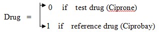
Real data was obtained from “The Pharmacy Services Unit”, Faculty of Pharmacy, University of Alexandria. The dataset consists of two drugs (test and reference), each contains ciprofloxacin substance which is known to be used for nausea, vomiting, headache, skin rash, etc. Test drug is the Ciprone tablet which contains 500 mg ciprofloxacin per tablet and produced by the Medical union pharmaceuticals Co., Abu Sultan-Ismailia, Egypt. Reference drug is the Ciprobay tablet, which contains 500 mg ciprofloxacin per tablet and produced by Bayer AG., Germany. Data represents plasma blood levels of ciprofloxacin (mg/ml) of 28 healthy human male volunteers, their ages ranged from 20 to 40 years and their weights ranged from 61 to 85 kg. Volunteers were divided into two equal groups. The first group of volunteers was administrated a single dose of 500 mg ciprofloxacin as one Ciprone tablet (test product), while the second group was administrated the same dose of ciprofloxacin as one Ciprobay tablet (reference product). After one week wash-out period, the first group of volunteers was administrated one tablet of Ciprobay (reference product), while the second group was administrated one tablet of Ciprone (test product). Venous blood samples (5 ml) were taken from each volunteer at times 0.5, 1.0, 1.5, 2.0, 2.5, 3.0, 3.5, 4.0, 6.0, and 8.0 hours after each dose. This data can be represented in a binary form model where the test drug (Ciprone) will be given a zero value, and the reference drug (Ciprobay) will be given a value of one as follows:
 (8)
(8)
Our goal here is to test if there is a significant difference between test and reference drugs on plasma levels of ciprofloxacin at different times. The binary response variable is “Drug”, and the times 0.5, 1.0, 1.5, 2.0, 2.5, 3.0, 3.5, 4.0, 6.0, and 8.0 are the predictors. The underlying dataset was analyzed using an IBM-Compatible PC computer with a 700 MHZ AMD-Processor. The three statistical software packages are the SAS system for windows version 8.0, the SPSS for windows version 10, and MINITAB Release 13.2.
2.1 SAS OUTPUT
SAS has a variety of options that can be used to analyze data with binary response (dichotomous) variable. SAS uses the PROC statement to execute the required task. The response variable Drug is 0 or 1 binary (This is not a limitation. The values can be either numeric or character as long as they are dichotomous), and the times 0.5, 1.0, 1.5, 2.0, 2.5, 3.0, 3.5, 4.0, 6.0, and 8.0 are the regressors of interest, which will be written as T05, T10, T15, T20, T25, T30, T35, T40, T60, and T80 in the INPUT statement because SAS variables can not be written with special character in the middle.
2.1.1 SAS Logistic regression
To fit a logistic regression, we can use the commands:
PROC LOGISTIC;
MODEL DRUG = T05 T10 T15 T20 T25 T30 T35 T40 T60 T80 / LINK = Link function; Run;
This option of the link function can be either logit; probit; normit; or cloglog (complementary log log function). SAS PROC LOGISTIC models the probability of Drug = 0 by default. In other words, SAS chooses the smaller value to estimate its probability. One way to change the default setting in order to model the probability of Drug = 1 in SAS is to specify the DESCENDING option on the PROC LOGISTIC statement. That is, to use PROC LOGISTIC DESCENDING statement. With the logit link function option we will get the following SAS output:
With a normit link function option we will get the following SAS output:
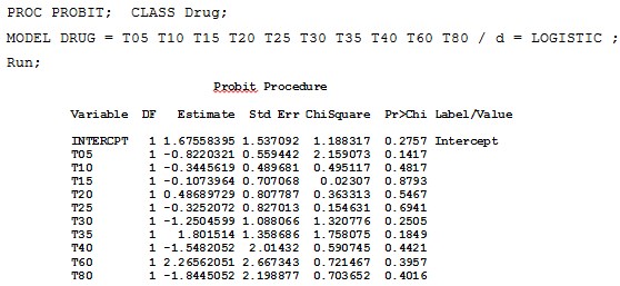
Similar results to the logit option can be obtained if we use the default of PROC PROBIT statement:
![]()
![]()
But this procedure does not show the odds ratio in its default.
2.1.2 SAS Probit regression
PROC PROBIT statement can be used to fit a logistic regression by specifying LOGISTIC as the cumulative distribution type in the MODEL statement. To fit a logistic regression model, we can use:
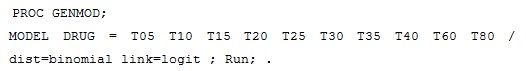
Logistic regression can also be modeled as a class of Generalized Linear Models by the GENMOD procedure, where the response probability distribution function is binomial and the link function is logit. The PROC GENMOD for a logistic regression, is:
Another type of SAS PROC statement is the SAS CATMOD (CATegorical data MODeling) procedure, which fits logistic regression as follows:
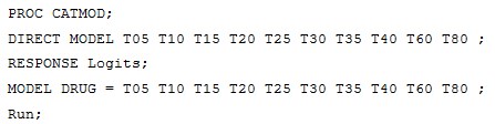
where the regressors are continuous quantitative variables and must be specified in the DIRECT statement. These procedures will give the same results as in the PROC LOGISTIC with no odds ratios in the output.
2.1.3 Complementary log-log
If we use the PROC LOGISTIC; with the option of link function = cloglog (Complementary log-log), we will get the following portion of SAS output:
2.2 SPSS OUTPUT
Unlike SAS procedure, the SPSS procedure LOGISTIC REGRESSION models the probability of Drug = 1 or higher sorted value by default. In other words, SPSS chooses the higher value to estimate its probability, while on the contrary SAS uses the smaller value.
2.2.1 SPSS Logistic regression
To fit SPSS logistic regression, we can use either the menu of BINARY LOGISTIC or ORDINAL REGRESSION.
Binary Logistic can be obtained from the Analyze menu, and selecting Regression option and from Regression menu select Binary Logistic. In the Binary Logistic dialog box select the variable Drug as a dependent variable and the times T0.5, T1.0, T1.5, T2.0, T2.5, T3.0, T3.5, T4.0, T6.0, and, T8.0 as covariates which will give the following portion of SPSS output:
PLUM — Ordinal Regression
Ordinal regression can be used to model the dependence of a polytomous ordinal (PLUM) response on a set of predictors, which can be factors or covariates. Ordinal regression can be obtained from the Analyze menu, then selecting Regression option and from Regression menu select Ordinal regression. In the Ordinal regression dialog box select the variable Drug as a dependent variable and the times T0.5, T1.0, T1.5, T2.0, T2.5, T3.0, T3.5, T4.0, T6.0, and, T8.0 as covariates, and choose Logit from the options to get the following SPSS output:
3.2.2 SPSS Probit regression
To fit SPSS Probit regression, we can use the menu of ORDINAL REGRESSION as before with the selection of Probit from the options to get the following SPSS OUTPUT:
2.2.3 SPSS Complementary log-log
In a similar way, we can use the menu of ORDINAL REGRESSION as before with the selection of Complementary log-log from the options to get the following SPSS OUTPUT:
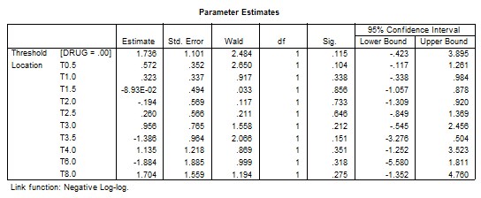
However, if we use the same menu of ORDINAL REGRESSION as before but with the selection option of Negative log-log we will get the following SPSS OUTPUT:
2.3 MINITAB OUTPUT
Minitab provides three link functions that can be used to fit binary response models. These functions are the logit, which is the default, the normit (probit), and the gompit (complementary log-log). These link functions can be obtained from the Stat menu, and by selecting the Binary Logistic Regression. In the Binary Logistic dialog box choose the variable Drug as the response variable and in the Model box select the times T0.5, T1.0, T1.5, T2.0, T2.5, T3.0, T3.5, T4.0, T6.0, and, T8.0 as the covariates. To specify the link function type, click in front of the required link function from the options box. This will give the following Minitab output:
2.3.1 Minitab Logistic regression
Selecting the option of logit link function, we will get the following portion of Minitab Binary Logistic Regression.

2.3.2 Probit regression
Binary Logistic Regression with the normit link function gives the following part of Minitab output:
2.3.3 Complementary log-log
Gompit link function with the Binary Logistic Regression gives the following portion of Minitab output:
3. INTERPRETATION OF THE STATISTICAL FINDINGS
Using the three statistical software packages SAS, SPSS, and Minitab to estimate the three specified models, Logistic regression model, Probit regression model, and the Complementary log-log model gave the following results:
3.1 SAS RESULTS
SAS gives three different sets of results with three different link functions, logit, normit, and Complementary log-log.
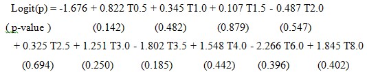
3.1.1 Logit Link Function
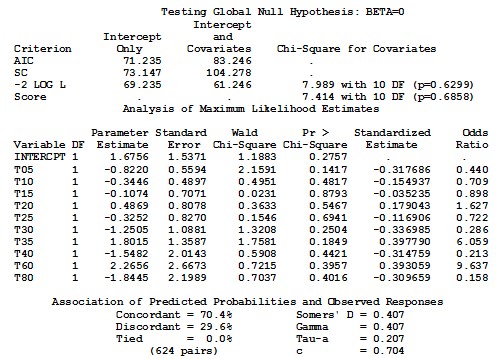
The output of the logit function can be obtained by either PROC LOGISTIC as a default, or by the determination of logistic distribution option in the PROC PROBIT, PROC GENMOD, and PROC CATMOD. Response Information displays 6 missing observations and the number of observations that fall into each of the two response categories are, 26 for the Test drug, and 24 for the Reference drug. Next, the –2 log-likelihood (–2 LOG L) from the maximum likelihood iterations is displayed along with the Chi-Square statistic. This statistic tests the null hypothesis that all the coefficients associated with predictors equal zero versus these coefficients not all being equal to zero. In the plasma blood levels data, c2 = 7.989, with 10 degrees of freedom and a p-value of 0.6299, indicating that there is no sufficient evidence that any one of the coefficients is different from zero, which means that there is no significant difference of plasma blood levels of ciprofloxacin between test and reference drug at the specified different times.
SAS output shows that the estimated logit link function:
Logit(p) = B0 + B1 T0.5 + B2 T1.0 + B3 T1.5 + B4 T2.0 + B5 T2.5 + B6 T3.0
+ B7 T3.5+ B8 T4.0+ B9 T6.0+ B10 T8.0 … (9)
is:
 (10)
(10)
where, p is the probability of the test drug = Prob(Drug = 0).
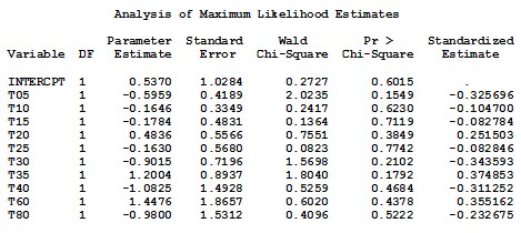
From the analysis of maximum likelihood Table we can find the estimated coefficients (parameter estimates), standard error of the coefficients, Wald’s Chi-Square values, p-values, standardized estimate, and the odds ratio. Testing the null hypothesis that each coefficient equal to zero, i. e., H0 = Bi = 0 for i = 1,2,..., 10. Results shows that the p-value for every coefficient is not less than a = 5 %, which means that none of the predictors is significant.
The estimated coefficients represent the change in the log odds for one unit increase in times. The odds ratio is the ratio of odds for one unit change in time. The odds ratio can be computed by exponentiating the log odds, i.e. EXP(log odds) or EXP(estimated coefficient), which is EXP(-0.822) = 0.440 for T0.5, and equal to EXP(-0.3446) = 0.709 for T1.0 and so on.
Association of predicted probabilities and observed responses are given in the last Table of the output. The number of concordant, discordant, and tied pairs is calculated by pairing the observations with different response values. Here, we have 26 observation of the Test drug and 24 of the Reference drug, resulting in 26 * 24 = 624 pairs with different response values. In this data, 70.4 % of pairs are concordant and 29.6 % are discordant. Somers’ D, Goodman-Kruskal Gamma, Kendall ’ s Tau-a, and c-correlation are summarized in the same table. These measures most likely lie between 0 and 1 where larger values indicate that the model has a better predictive ability. In this data, the measures are 0.407, 0.407, 0.207, and 0.704 respectively which implies less than desirable predictive ability.
3.1.2 Normit Link Function
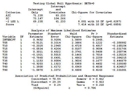
The normit link function is the inverse of the cumulative standard normal distribution function, and can be obtained by using the option normit in the PROC LOGISTIC statement. Response Information is the same as for the logit output. The Chi-square test statistic for testing the null hypothesis that all the coefficients associated with predictors equal zero is c2 = 8.001, with a p-value of 0.6287, indicating that there is no sufficient evidence that any one of the coefficients is different from zero, which means that there is no significant difference of plasma blood levels of ciprofloxacin between test and reference drug at the specified different times.
The estimated normit link function is:
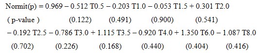 (11)
(11)
where, p is the probability of the test drug = Prob(Drug = 0).
We have similar output from the table of the maximum likelihood estimates. The estimated coefficients, standard error of the coefficients, Wald’s Chi-Square values, p-values, standardized estimate, and there is no odds ratio. We also obtained similar results when testing the null hypothesis that each coefficient equal to zero, i. e., H0 = Bi = 0 for i = 1,2,..., 10. The p-value for every coefficient is not less than a = 5 %, which means that all predictors are not significant.
Association of predicted probabilities and observed responses are given in the last Table of the output. The number of concordant, discordant, and tied pairs is 624 pairs with different response values. 70.5 % of pairs are concordant and 29.3 % are discordant. Somers’ D, Goodman-Kruskal Gamma, Kendall ’ s Tau-a, and c-correlation are summarized in the same table of SAS output. These measures 0.412, 0.413, 0.210, and 0.706 respectively which means that we do not have a very strong predictive ability of this model.
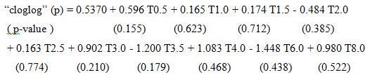
3.1.3 The Complementary log-log Link Function
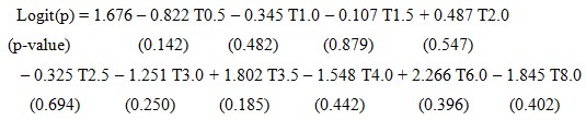
The complementary log-log (gompit/cloglog) link function is obtained by using the option “cloglo” in the PROC LOGISTIC statement. Response Information is the same as for the logit and normit output. The Chi-square test statistic for testing the null hypothesis that all the coefficients associated with predictors equal zero is c2 = 7.721, with 10 degrees of freedom and a p-value of 0.6560, indicating that there is no sufficient evidence that any one of the coefficients is different from zero, which means that the effect of test (Ciprone) and reference (Ciprobay) drug is the same on plasma blood levels of ciprofloxacin at the specified different times. The estimated complementary log-log “cloglog” link function is:
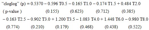 (12)
(12)
where, p is the probability of the test drug = Prob(Drug = 0).
From the Table of the maximum likelihood estimates, we can find the estimated coefficients (parameter estimates), standard error of the coefficients, Wald’s Chi-Square values, p-values, and the standardized estimate. Testing the null hypothesis that each coefficient equal to zero, i. e., H0 = Bi = 0 for i = 1,2,..., 10. Results are similar to the previous cases, where the p-value for every coefficient is greater than 5 %, which means that all predictors are not significant.
Association of predicted probabilities and observed responses reveals that he number of concordant, discordant, and tied pairs is 624 pairs with different response values. 71.0 % of pairs are concordant and 28.8 % are discordant. Somers’ D, Goodman-Kruskal Gamma, Kendall ’ s Tau-a, and c-correlation are 0.421, 0.422, 0.215, and 0.711 respectively which means that we do not have a very strong predictive ability of this model.
3.2 SPSS RESULTS
SPSS is similar to SAS, where SPSS gives three different sets of results with three different link functions, logit, normit, and Complementary log-log.
3.2.1 Logit Link Function
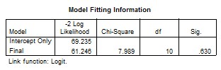
The output of the logit function can be obtained by either Binary Logistic Regression menu as a default, or by the determination of logistic distribution option in the Ordinal Regression menu. The main advantage of the Binary Logistic Regression command is that, we get the odds ratio beside the regular output. From the Binary Logistic Regression output, we can find the Case processing summary, which indicates that we have 56 cases with 6 missing cases. In the initial classification table there are 26 for the Test drug, and 24 for the Reference drug. The omnibus tests of the model coefficients shows that the Chi-square test statistic for testing the null hypothesis that all the coefficients associated with predictors equal zero is c2 = 7.989, with 10 degrees of freedom and a p-value of 0.630, which is the same result obtained by SAS. The classification table of SPSS output, shows that we have 74 % of correct classification.
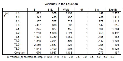
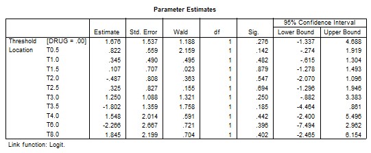
From the variables in equation table we can find the estimated coefficients (B), standard error of the coefficients (SE), Wald’s Chi-Square values, Degrees of freedom (df), p-values (Sig), and the odds ratio {Exp(B)}. The estimated SPSS logit link function is:
 (13)
(13)
The difference between Equation (10) of SAS and Equation (13) of SPSS output, is that, they have an opposite corresponding signs, that is because, SAS considers the probability p = Prob(Drug = 0) which is the probability of the test drug, as its default, while SPSS considers p = Prob(Drug = 1) which is the probability of the reference drug, as its default. That is why the odds ratio of SPSS output is shown as the reciprocal of the odds ratio of SAS output. The computation of the odds ratio is EXP(log odds) or EXP(estimated coefficient), which is EXP(-0.822) = 0.440 for T0.5 using SAS, while the odds ratio is EXP(0.822) = 2.275 = 1/{EXP(-0.822)} = 1/0.440 for the same time T0.5 using SPSS. Also, the odds ratio is EXP(-0.345) = 0.709 for T1.0 using SAS, while when using SPSS, the odds ratio is EXP(0.345) = 1.411 = 1/{EXP(-0.345)} = 1/0.709 for the same time T1.0, and so on for the other odds ratio.
Additional output results are provided by SPSS when we use the logit as a link function option. Goodness of fit information is given for Pearson and Deviance tests using the Chi-square test statistic, c2 = 49.795, with 39 degrees of freedom and a p-value of 0.115 for the Peasron test, and c2 = 61.248, with 39 degrees of freedom and a p-value of 0.013 for the Deviance test. Also, a 95 % confidence interval is provided for every parameter. According to Pearson’s result only, we can conclude that the model fits data adequately, because the p-value = 11.5 % which is less not than 5 %.
3.2.2 Normit Link Function
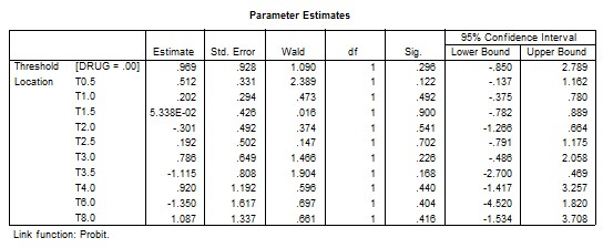
The normit link function is obtained from the probit regression option in the ordinal regression menu. It provides the inverse of the cumulative standard normal distribution function. From the model fitting information, the Chi-square test statistic for testing the null hypothesis that all the coefficients associated with predictors equal zero is c2 = 8.001, with 10 degrees of freedom and a p-value of 0.629, indicating that we fail to reject the null hypothesis. SPSS parameter estimates of the normit link function is:
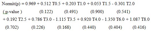 (14)
(14)
Equation (14) of SPSS is the same as Equation (11) of SAS, but with opposite signs for the estimated coefficients, because, p which is the probability of the reference drug = Prob(Drug = 1) as a default of SPSS. Goodness of fit information is given for Pearson test, c2 = 49.506, with df = 39 and a p-value of 0.121, and for the Deviance test c2 = 61.233, with df = 39 and a p-value of 0.013.
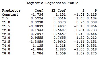
3.2.3 The Complementary log-log Link Function
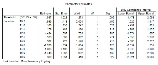
The complementary log-log link function is obtained by selecting it from the ordinal regression menu. Model fitting information table shows that c2 = 7.721, with 10 degrees of freedom and a p-value of 0.6560, indicating that there is no sufficient evidence that any one of the coefficients is different from zero, which is the same result as SAS. The estimated “cloglog” link function is:
 (15)
(15)
Equation (15) of SPSS is the same as Equation (12) of SAS, but again with opposite signs for the estimated coefficients, because, p which is the probability of the reference drug = Prob(Drug = 1) as a default of SPSS. Goodness of fit information is given for Pearson and Deviance tests using the Chi-square test statistic, c2 = 48.936, with df = 39 and a p-value of 0.132, while for the Peasron test, and c2 = 61.513, with df = 39 and a p-value of 0.012 for the Deviance test. Also, a 95 % confidence interval is provided for every parameter. It worth noting that SPSS does not provide any information about association of predicted probabilities and observed responses as we found in the SAS output.
3.3 MINITAB RESULTS
Minitab gives different sets of results for the three link functions the logit, which is the default, the normit (probit), and the gompit (complementary log-log) by selecting the Binary Logistic Regression from the Stat menu.
3.3.1 Logit Link Function
Minitab results looks like a combination of SAS and SPSS output, where Minitab output for the logit link function includes a response information table exactly as in SAS output, logistic regression table very similar to SPSS, goodness of fit table similar to SPSS, and measures of association very similar to SAS. Response information table shows that we have 26 event for the reference drug and 24 for the test drug. Logistic regression table provides the estimated coefficients (Coef), standard error of the coefficients (SE Coef), Z values, p-values, odds ratio, and 95 % CI’s for the B’s. The estimated Minitab logit link function is exactly as Equation (13) of SPSS output. Testing the null hypothesis that all slopes are zero, is done through a G test, which gives the same results as SPSS. Also, testing, H0 = Bi = 0 for i = 1,2,..., 10 is the same with same conclusions of SPSS and SAS although it is done using the normal approximation and the Z test.
A 95 % confidence interval is provided for every parameter. The values of these CI’s are different from SPSS because they are computed using the normal approximation and the standard normal Z-table, while SPSS uses the chi-square tables. The odds ratios calculated by Minitab are exactly as SPSS results.
Pearson and Deviance tests are provided by Minitab as well as by SPSS as tests for goodness of fit. In addition to Pearson, Deviance Minitab calculates Hosmer-Lemeshow tests. The Chi-square test statistic, c2 = 49.795, with df = 39 and a p-value of 0.115 for the Peasron test, c2 = 61.248, with df = 39 and a p-value of 0.013 for the Deviance test, and c2 = 5.820, with df = 8 and a p-value of 0.667 for the Hosmer-Lemeshow test.
Very similar to SAS, association of predicted probabilities and observed responses are given in the last table of Minitab output. The number of concordant, discordant, and tied pairs is 624 pairs. 70.2 % of pairs are concordant and 29.5 % are discordant. Somers’ D, Goodman-Kruskal Gamma, and Kendall ’ s Tau-a are summarized in one table of Minitab output. These measures are 0.41, 0.41, and 0.21 respectively.
3.3.2 Normit Link Function
The normit link function is obtained through the probit regression option using Minitab. Response information table is exactly as in SAS output. The logistic regression table provides the estimated coefficients, the standard error of the estimates, the Z and p- values for every estimates. The estimated normit link function is exactly as Equation (14) in SPSS output with one exception, where the constant term has a negative sign opposite to SPSS result. Testing that all slops are zero, is exactly the same as SAS and SPSS. Goodness of fit is similar to SPSS but with the addition of Hosmer-Lemeshow, where c2 = 5.927, with df = 8 and a p-value of 0.655, which means that the model fits data adequately.
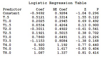
3.3.3 The Complementary log-log Link Function
Surprisingly the Minitab output of the complementary log-log link function is completely different from the corresponding output of both SAS and SPSS. The estimated “cloglog” link function is:
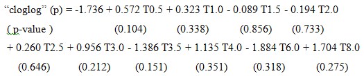 (15)
(15)
Consequently, all goodness of fit tests, and measures of association are different from SAS and SPSS. The G-test for testing that all slopes are zero is 8.685 with df = 10 and p-value 0.562. The Chi-square test statistic for testing goodness of fit is c2 = 50.284, with df = 39 and a p-value of 0.106 for the Peasron test, c2 = 60.550, with df = 39 and a p-value of 0.015 for the Deviance test, and c2 = 6.427, with df = 8 and a p-value of 0.600 for the Hosmer-Lemeshow test. Measures of association of predicted probabilities and observed responses show that, number of concordant, discordant, and tied pairs is 624 pairs. 71.5 % of pairs are concordant and 28.2 % are discordant. Somers’ D, Goodman-Kruskal Gamma, and Kendall ’ s Tau-a are 0.43, 0.43, and 0.22 respectively.
It worth noting that this Minitab results of the complementary log-log link function can be obtained exactly using SPSS but with the selection of the Negative log-log option as previously shown in the SPSS output.
Table 2
Comparison between SAS, SPSS, and MINITAB
|
Criterion |
SAS |
SPSS |
MINITAB |
|
Model fitting: testing all B’s = 0 |
Same result |
Same result |
Same result |
|
Values of the estimated parameters |
Same values |
Same values |
Same values |
|
Signs of the estimated parameters |
Opposite signs |
Same signs |
Same signs |
|
Odds ratio |
EXP(Bi) |
1/{EXP(Bi)} |
1/{EXP(Bi)} |
|
C.I’s for the B’s |
X |
Calculated using Wald’s c2 |
Calculated using Z-values |
|
Goodness of fit tests |
X X X |
Pearson test Deviance test X |
Pearson test Deviance test Hosmer-Lemeshow test |
|
Measures of Association |
Concordant & Discordant pairs. Somers’D Gamma Kendall’s Tau-a C |
X X X X X |
Concordant & Discordant pairs. Somers’D Gamma Kendall’s Tau-a X |
|
Default for the binary response variable y |
P(y = 0) |
P(y = 1) |
P(y = 1) |
(X) Means not available by default.
References:
1. McClenahan, C.L. “Ratemaking.” In Foundations of Casualty Actuarial Science, Fourth Edition. Arlington, VA: Casualty Actuarial Society, 2000.
2. McNeil, A.J., Frey, R., and Embrechts, P. Quantitative Risk Management: Concepts, Techniques and Tools. Princeton, NJ: Princeton University Press, 2005.
3. Phillips, R. L. Pricing and Revenue Optimization. Stanford, CA: Stanford University Press, 2005.
4. Ramsay, C.M. “A system of integro-differential-difference equations in risk theory, using compound birth-death processes.” Scandinavian Actuarial Journal (1985): 39–48.
5. Sandstrom, A. “Solvency II: calibration for skewness.” Scandinavian Actuarial Journal (2007): 126–134.
